TL;DR. A number-guessing game leads directly to the main quantities used in information theory and language-model training: halve the space → log₂N questions → the bit → questions as codes → −log₂p per outcome → entropy → conditional entropy → cross-entropy and perplexity → KL divergence → forward and reverse KL.
Start with a game.
I chose a number between 1 and 100. Try to find it with as few guesses as possible. After each guess, I will only say whether the number is higher or lower.
I'm thinking of a number between 1 and 100.
Make your first guess.
Guesses: 0
still possibleruled out
Play a few rounds. The strip shows what you still don't know: white cells are still in play, grey cells have been ruled out.
The best strategy for this game is also the starting point of information theory.
The same idea later appears in coding, compression, and machine-learning loss functions.
What is the optimal strategy?
If the number is uniform, the chance of guessing it immediately is:
$$P(x) = \frac{1}{100}$$
A wrong guess can still narrow the search. Suppose the guess is 71. The three possible outcomes are:
$$
\begin{aligned}
P(x = 71) &= \tfrac{1}{100} &&\longrightarrow\; \text{0 numbers left to search} \\[6pt]
P(x < 71) &= \tfrac{70}{100} &&\longrightarrow\; \text{70 numbers left to search} \\[6pt]
P(x > 71) &= \tfrac{29}{100} &&\longrightarrow\; \text{29 numbers left to search}
\end{aligned}
$$
x < 71 (70 numbers)
71
x > 71 (29)
1100
Guessing 71 cuts the line into two very uneven pieces. Most of the time (70%) you land in the big chunk on the left and have barely narrowed anything down.
Weighting each outcome by its probability gives the expected number of candidates left:
After one guess, we expect to have 57.41 numbers still left to check. We started with 100 and, on average, more than half are still on the table. For a single question, that is a poor return.
To minimize the expected number left, keep the guess as a variable $x$ and solve for its optimum:
Step 1. Write the expected number left, weighting each outcome by its probability:
This is a parabola in $x$, so its minimum occurs where the derivative is zero:
Step 1. Differentiate each square with the chain rule, $\;\frac{d}{dx}(100-x)^2 = -2(100-x)$:
$$E'(x) = \frac{2(x-1) - 2(100-x)}{100}$$
Step 2. Set it to zero and multiply both sides by 100:
$$2(x-1) - 2(100-x) = 0$$
Step 3. Divide by 2:
$$(x-1) - (100-x) = 0$$
Step 4. Drop the parentheses, watching the signs:
$$x - 1 - 100 + x = 0$$
Step 5. Collect terms:
$$2x - 101 = 0$$
Step 6. Solve for $x$:
$$x = \frac{101}{2} = 50.5$$
Since the number is a whole number, that means guessing 50 or 51: the middle. Plugging it back in, the expected number left drops to
$$E(50) = \frac{49^2 + 50^2}{100} = 49.01$$
Compare that to the 57.41 we got from guessing 71. The middle is the most informative guess we can make, because it splits the remaining numbers as evenly as possible: whatever answer comes back, we throw away half the space.
After that first guess, we are left with about 50 numbers and the exact same problem, just smaller. So we do the same thing again: ask the middle, halve it again. And again.
How Many Questions Are Necessary?
Each answer is binary: higher or lower. The best question splits the remaining candidates in half, so either answer removes half of them.
The minimum number of questions is therefore the number of times 100 can be halved before one candidate remains. That is the base-2 logarithm:
$$\log_2(100) \approx 6.64$$
This means 6.64 ideal halving questions. A single game still needs a whole number, so seven questions are enough in the worst case. Six questions distinguish only $2^6 = 64$ outcomes, while seven distinguish $2^7 = 128$. The average cost can still lie between six and seven.
A smaller game makes the fractional average easier to see. The tree below sends the lower half left and the upper half right at each split. The depth of a number is its question count.
The game runs from 1 to 10
The halving game, small enough to see whole. Each split sends the lower half left (a 0) and the higher half right (a 1), so every number ends up with a 0/1 codeword whose length is how many questions it took. At a power of 2 the bottom is one clean row and log₂N is a whole number; everywhere else it goes ragged, a few numbers needing one extra question. That raggedness is what a fractional log₂ means.
Two things to notice. Land on a power of 2, like 8 or 16, and the tree is a perfect block: every number sits on the same bottom row, and log₂N is exactly a whole number. Step off it, and the bottom goes ragged. Some numbers get pinned down a row early, the rest need one more question, and the average always settles above log₂N. For 100 the very same raggedness happens between rows 6 and 7, which is the 6.64 we could not round away.
The tree puts a number on something else, too: how often you actually pay for that extra question. For 100, the deep row holds 72 of the numbers and the shallow row holds 28, so 72% of the time you end up asking the 7th question, and 28% of the time you are done at 6. Weigh those and the true average is $0.72 \times 7 + 0.28 \times 6 = 6.72$ questions.
That 0.72 is worth a second look, because it is not the 0.64 from $\log_2 100 = 6.64$. The 0.64 is the ideal, what one number in a hundred would cost if questions could come in fractions. The 0.72 is what you actually pay, nudged higher because the deepest numbers always come in pairs: every split sends two of them down, so the deep row holds an even count that slightly overshoots the ideal. The difference, $6.72 - 6.64 = 0.08$ of a question per game, is the waste: the toll for asking in whole questions, and it vanishes exactly when N is a power of 2.
This is the gap Claude Shannon closed in 1948. The thing that genuinely equals 6.64 is not a number of questions, it is an amount of information, and information has no reason to come in whole questions. Shannon gave it a unit: the bit. One bit is the information carried by a single perfect yes-or-no answer, the answer to a 50/50 question, and each 0 or 1 in the codewords above is exactly one bit. Measured that way, learning which of 100 equally likely numbers I picked is worth $\log_2(100) \approx 6.64$ bits. You round the questions up to 7, but the information was 6.64 bits all along.
The simulation below compares halving with a baseline that splits the remaining range at a random point. Over thousands of games, halving settles near the predicted 6.72 questions while the random baseline stays higher.
Games played: 0
Halving (optimal)this game: 0 q · avg –
Random split (baseline)this game: 0 q · avg –
Each strategy plays thousands of games. The bars show one game in progress narrowing toward the answer; the plot tracks the running average number of questions. Halving hugs the log₂100 floor from above, while random splitting wastes its questions on lopsided cuts.
Two things happen. The random baseline drifts up to around 8.4 questions per game, about a quarter more than it needs, because it keeps making lopsided cuts that barely shrink the space. Halving settles right around 6.7, and it never dips below the $\log_2(100)$ line.
Exercise. That 8.4 is not a quirk of the simulation. Show that for $n$ equally likely numbers, the random-split strategy needs on average $2(\mathcal{H}_n - 1)$ questions, where $\mathcal{H}_n = 1 + \tfrac{1}{2} + \tfrac{1}{3} + \cdots + \tfrac{1}{n}$ is the $n$-th harmonic number. (Hint: condition on where the first random split lands and set up a recurrence.) For $n = 100$ this works out to about 8.37. The full derivation is in the appendix.
$\log_2(100)$ is a lower bound, not just the score of one strategy. Halving reaches 6.72 questions on average. The 0.08-bit gap above the bound comes from using whole questions.
Finding one of 100 equally likely outcomes costs at least 6.64 bits. The next section shows why no strategy can beat that bound.
From questions to codes
So far, we have come to halving as our best strategy, with empirical direction motivating it. But are there any better strategies?
Every time you play, the answers you collect are a string of yes-or-nos, which we have been writing as 0s and 1s. Trace any number down the tree and you get its string: in the game from 1 to 16, the number 11 comes out as 1010, the number 3 as 0010, and every number has its own. The string is enough to rebuild the number, too. Hand someone the bits 1010 and, walking the same tree, they land on 11 with nothing else to go on.
(A note for anyone who counts from zero: because our numbers start at 1, the codeword for the $k$-th number is the binary of $k-1$. So 0000 is the number 1, not 0, and the last bit flips the usual odd/even rule. Nudge your index by one and it all lines up; nothing in the argument depends on where we start counting.)
So the game was never really about questions. It was about encoding. The tree assigns every number a codeword, and reading off the codeword is the same as naming the number. A friend who knows the tree can take your bits and recover exactly what you meant.
number
11
encode →
1010
transmit →
1010
decode →
number
11
The questions were a communication channel all along. The codeword is the message; sending it sends the number.
Once you see it as a code, "best" finally has a precise meaning. The best strategy is the one that, on average, sends the shortest messages. So: is halving really the shortest code, or could something cleverer do better?
The code you would have written anyway
Suppose I asked you to encode the numbers 1 to 16 in bits. You would not draw a tree. You would just count in binary: 0000, 0001, 0010, all the way to 1111. Sixteen numbers, four bits each, done.
Here is the surprise: that is exactly the halving code. Slide the tree above to 16 and look. Every codeword is four bits, and they are the binary numerals in order. When the count is a power of 2, the obvious fixed-width encoding and the clever halving strategy are the same thing. You had already invented it.
The two only part ways when the count is not a power of 2. Slide the tree to 15. Fixed-width can do nothing clever: 15 still needs 4 bits, because 3 bits can only address 8 things, so every number costs 4. But halving hands a 3-bit codeword to one of the numbers and 4 bits to the rest, averaging 3.93. It compresses, by refusing to spend a bit it does not need.
How far can that go? The two codes agree on every number but the last, so the whole saving is hiding in what happens to 15:
fixed-widthhalving (ours)100000000200010001⋮identical⋮1411011101151110111(16th)1111never made
Identical for 1 through 14. They split only on 15: fixed-width writes 1110, holding it apart from a sixteenth number (1111) that never arrives, while halving sees that slot is empty and drops the final bit, leaving 111. That one struck bit is the entire difference between the codes.
Averaged over all fifteen numbers, that single saved bit is the whole story, and it lands just shy of the information floor:
Halving claws back almost all of the slack that fixed-width wastes, and stops right before the floor, that last 0.02 being the same integer-codeword tax we have already met. (You can chip at it by bundling several numbers into one codeword, but that is a story for another day.)
But 15 was the 'worst' case in its range: only one number sat shallow enough to save a bit. Swing to the other extreme, to just above a power of 2, and observe. Here is 1 to 9:
Just above a power of 2, the saving flips. Seven of the nine numbers now get a 3-bit codeword (green); only 1 and 2 still need the fourth bit. Fixed-width spends 4 bits on all nine.
That is nearly the whole bit saved on nearly every number. Fixed-width still costs a flat 4.00 bits; halving averages 3.22, against a floor of $\log_2 9 \approx 3.17$.
Either way, halving beats the naive encoding. But beating the naive code is a low bar. Could some genuinely clever code beat halving?
Why nothing can beat it
Any predictable pattern in a code's output is redundancy. If the next bit can be guessed better than chance, a shorter code can avoid spending bits on what was already predictable.
Turn that around. The optimal code is the one whose output you cannot compress, because there is no pattern left to exploit. Its bits look like fair coin flips: each one equally likely 0 or 1, independent of the last, every block as common as every other. The endpoint of squeezing all the redundancy out of a message is something indistinguishable from noise.
pure coin flips
halving (our code)
guess low (wasteful)
Each square is several thousand yes-or-no answers, drawn as black-and-white pixels. Coin flips and the halving code are statistically identical: genuine static, with nothing left to compress. The wasteful "guess low" strategy gives itself away, so many of its answers are foregone conclusions that the square fades pale. An optimal code's output is, quite literally, indistinguishable from randomness.
Only noise is incompressible
Structure is exactly what compression feeds on. A message you can shorten still has predictability left in it. When nothing can shorten it any further, what remains looks completely random, which is why a perfectly encoded message and pure noise are impossible to tell apart.
Halving produces this kind of stream. Every answer is 50/50 and carries a full bit. A lopsided question, such as asking whether the number lies in the bottom quarter, produces a partly predictable answer and wastes part of the question.
There is a hard floor underneath the intuition, too. A single yes-or-no answer can carry at most one bit. Identifying one number out of $N$ equally likely ones takes $\log_2 N$ bits. So no strategy, however clever, can use fewer than $\log_2 N$ questions on average. Halving extracts a full bit from every even split, so it presses right up against that floor, and nothing can do better.
The picture catches the gross cases, but the eye is a blunt instrument. A mildly off-center strategy wastes only a little, and its square would still look like static. To catch waste too small to see, we stop looking and start counting.
The fingerprint of a perfect code
We can test this by playing thousands of games from 1 to 16 and joining the answers into one bit stream. For an optimal code, individual bits, pairs, and triples should appear at equal rates. A wasteful strategy produces uneven counts.
strategy
pattern length
Every yes-or-no answer from thousands of games of 1-to-16, counted as patterns. Bars on the dashed line mean every pattern is equally likely: the mark of a code with nothing left to compress. Bars that lean are wasted predictability.
The optimal code's bars sit flat on the line: every pattern equally likely, no structure, nothing to compress. Push to off-center and the bars start to lean. Push to guess low and they collapse into a heap of 1s, an answer so predictable it is barely worth asking. That lean is the redundancy, and the readout above turns it into a number: a full bit per answer when the code is perfect, less and less as the waste grows.
A sequence in which every block of length $k$ appears with frequency $1/2^k$ is called normal, following Borel (1909). A perfect code produces a normal stream in this sense. With 100 outcomes rather than a power of two, optimal halving is only almost flat. The remaining bias corresponds to the same 0.08-bit overhead caused by whole questions.
The price of a single outcome
We have one more thing to harvest, and it is the key to everything that follows. All along, the length of a codeword has been shadowing a probability. A codeword that is $n$ bits long singles out one message among $2^n$ equally likely ones, so the chance of any particular $n$-bit message is
$$p = \frac{1}{2^n} = 2^{-n}$$
Read it backwards to get the length from the probability:
Step 1. Take the base-2 log of both sides:
$$\log_2 p = \log_2 2^{-n} = -n$$
Step 2. Flip the sign:
$$n = -\log_2 p$$
So an outcome that happens with probability $p$ costs $-\log_2 p$ bits to name. That single formula is the whole game. Check it against everything we have done: one number out of 100 equally likely ones has $p = 1/100$, so it costs
which is exactly the number we started with. Our entire story so far has been the special case where every outcome shares the same probability $1/N$, handing every outcome the same price $\log_2 N$.
Step back and look at what we have built, because it is the whole foundation. A bit is the answer to one maximally informative question, and a question is most informative exactly when you are most uncertain of its answer: when it is framed so that yes and no are equally likely, each with probability one-half. That coin-flip question is worth a full bit. Tilt the odds and the answer turns partly predictable, so it pays out less. The bits it takes to pin something down are just the count of those balanced questions, and an outcome of probability $p$ takes exactly $-\log_2 p$ of them.
And that last formula asks only about a single outcome's own probability; it never counts how many outcomes there are, and never insists they be equally likely. We have only ever used it on fair games, where every outcome shares the same $p = 1/N$.
From a bit to entropy
The buildup to what a bit is, and why it is the same thing as information, may have felt long. That was deliberate. The goal so far was to make the idea intuitive and to turn it over in the hand, to see it from the game, from the code, from the noise. From here we can move fast. Everything that follows falls straight out of that one idea, and if each step lands as the obvious next thing, the slow start did its job.
By now one claim should sit comfortably: a bit is a unit of information, and information is a measure of compression. But every example so far has been a fair, uniform draw, every outcome equally likely. Two questions are left hanging:
How do we picture a non-uniform distribution in the language of compression?
When we send a codeword, or a whole stream of them, how much should we expect to pay?
Picturing a non-uniform distribution
We already hold the answer; we just have to read it off. An outcome of probability $p$ costs $-\log_2 p$ bits to name, and that one rule is the entire bridge from probability to compression: a common outcome (large $p$) is cheap, a rare one (small $p$) is expensive. Lay the probabilities out as areas and you can see it at a glance. The wide blocks, the things that happen often, get the short codes.
The binary tree of every address. Each object's codeword carves out a region of it: 0 (object A) claims the whole left half, 10 (B) a quarter, 110 and 111 (C, D) an eighth each. The braces read off the width of each region, which is its probability; the depth, the number of bits, is its cost. A length-$L$ codeword owns $1/2^L$ of the tree, so the more likely the object, the wider its block and the shorter its code.
Nothing here was special about a guessing game. Strip away the story and what is left is a source: it emits objects $x$ from some set, each with its own probability $p(x)$, and a message is just a sequence of them, $x_1, x_2, x_3, \ldots$. Pixels in an image, letters in a sentence, states of the weather. Anything that carries a probability is information, and anything that is information can be compressed and sent. The cost of one object is its surprise, $-\log_2 p(x)$, whatever the object is and however many others there are.
What is the cost of a sequence?
Notice the word we keep leaning on: expect. We are not asking what one particular object costs, we are asking what it costs on average, per object, across a sequence. That is an expectation.
If you have met the entropy formula before and found it opaque, this is the form that makes it click:
$$H(X) = \mathbb{E}\!\left[-\log_2 p(X)\right]$$
Read it as plain words. The inside, $-\log_2 p(X)$, is the bit cost of whatever object we happen to draw. The $\mathbb{E}[\cdot]$ averages that cost over the source. To take the average, weight each object's cost by how often it turns up, and sum over every object:
That is entropy: a weighted average of the bit cost of each outcome, weighted by how often you actually see it. The common outcomes are cheap to name and dominate the sum because they happen so much; the rare ones are costly but seldom. The number that comes out is the average bits per object, and, exactly as before, it is a floor: the fewest bits, on average, that any code can spend to send one draw from this source.
And it contains everything we did. A fair game over $N$ outcomes has $p(x) = 1/N$ for every $x$, so every cost is the same, $-\log_2(1/N) = \log_2 N$, and the average of a constant is just that constant: $H = \log_2 N$. The uniform case was never a different rule. It was only the special case where every term in the sum agrees.
When the past predicts the future
We talk about bits, information, and entropy, but once again a major assumption has been hiding underneath: each event is independent. Now, I work on AI for a living, and if that is your world too, your mind is probably already jumping to LLMs. An LLM works autoregressively, and it is not only LLMs: in most settings where you want compression, there is dependence. A letter conditions the probability of the next one, and so does a word, a sentence, a pixel, a token.
So we no longer formalize only as $p(x)$, but as $p(x \mid \text{context})$, the conditional probability of $x$ given an existing context: a single letter, a word, a prompt. The surprise of the symbol that actually arrives is what it always was, its negative log probability, only now conditioned on the past:
When the context makes the symbol obvious, that surprise collapses. The u after a q has $p \approx 1$, so $-\log_2 p \approx 0$: it costs almost nothing to send, because you already knew it was coming. A whole sequence factorizes into these one-step predictions, each conditioned on its past, which is just the chain rule of probability:
And here is the fact that makes memory worth having: conditioning never hurts. On average, knowing the past can only lower your uncertainty about what comes next, so $H(X_t \mid X_{<t}) \le H(X_t)$. English taken letter by letter, as if each were independent, costs around four bits each; let the context speak and Shannon estimated the true figure at closer to one bit per letter. Something like three quarters of written English is, in this exact sense, redundant: already implied by what came before.
When you only have an approximation
You might have noticed we keep talking about a probability distribution $p$, but we also keep mentioning LLMs, and an LLM is only an approximator of the true language distribution. It never has $p$. This is why we introduce $q$, the learnt distribution, which tries to approximate $p$. And entropy, we saw, is built on $-\log_2 p$. So how do we calculate the entropy through our approximation $q$?
The real question is what it costs to compress with the wrong distribution: a code built for $q$ when the data actually comes from $p$. The answer is the natural one. You give each symbol the length your model thinks it deserves, $-\log_2 q(x)$ bits, but the symbols arrive with their true frequencies $p(x)$. So you average the $q$-cost over the real distribution $p$:
This is the cross-entropy: the average bits you spend encoding a source $p$ with a code meant for $q$. It is entropy with one factor swapped. The weight $p(x)$ is reality, how often a symbol really shows up; the cost $-\log_2 q(x)$ is the model's belief about it. When the model is right, $q = p$, and it collapses back into plain entropy. When it is wrong, the swap makes you pay.
For a language model this is the pretraining loss, nothing more. The model reads the context, predicts a distribution $q(x_t \mid x_{<t})$ over the next token, and pays $-\log_2 q$ on whatever token actually comes next; averaged over the data, that is the cross-entropy the optimizer drives down. (In practice the loss is reported in nats, using the natural log in place of $\log_2$; that only rescales everything by a constant factor of $1/\ln 2$, so every bit of intuition here carries over untouched.) Exponentiate it and you get perplexity, $2^{H(p,q)}$, the effective number of equally likely tokens the model is torn between at each step. A perplexity of 8 is as unsure as a fair eight-sided die.
A note on perplexity. Run the same computation the other way and it hands you an intuitive read on the difficulty of the task itself.
Say I am compressing one token sampled from a 100,000-word vocabulary. If the model estimates that token at 3 bits, then $2^3 = 8$ says that, as far as the model is concerned, the 100,000 options have shrunk to a choice among 8.
Now average it over the model's answers. Say the cross-entropy is 4.3 bits per token. Then $2^{4.3} \approx 19.69$: for each autoregressive step, the model is effectively branching among about 20 possible next tokens.
That is perplexity, $2^{H}$. You may wonder why we bother, since the bits already carry the same insight. The log scale is the better place to compute, surprises add instead of multiplying, but a linear count, "about 20 choices", is far easier for a human to feel than "4.3 bits".
How many extra bits?
The average number of extra bits paid for using $q$ instead of the true $p$ is the KL divergence, $D_{\mathrm{KL}}(p \,\|\, q)$.
If you have run into it before, you have probably seen it raw:
And suddenly KL is not some mysterious distance-like quantity. It is, literally, the expected wasted bits from holding the wrong model of reality. And since the true code is the cheapest one there is, the wrong code can only ever cost you more, never less: those wasted bits are always at least zero, $D_{\mathrm{KL}}(p \,\|\, q) \ge 0$, with equality exactly when $q = p$. (That is Gibbs' inequality, and it is the reason cross-entropy can never dip below entropy.)
It also shows cleanly why KL is a divergence and not a distance: it is asymmetric, $D_{\mathrm{KL}}(p \,\|\, q) \ne D_{\mathrm{KL}}(q \,\|\, p)$. In the compression reading, that asymmetry is the natural thing, not a defect. $D_{\mathrm{KL}}(p \,\|\, q)$ asks: reality is $p$, I built my code from $q$, how many extra bits do I waste? Whereas $D_{\mathrm{KL}}(q \,\|\, p)$ asks: if the samples were actually drawn from $q$, how many extra bits would a code built for $p$ cost?
The deeper reason they differ is that the measure you average against changes. Compare:
The first asks: where does reality spend its probability mass, and how wrong is my model there? The second asks: where does my model spend its mass, and how wrong am I there?
And this hands you a surprisingly deep reading of machine learning itself. Maximum likelihood training is the same thing as minimizing cross-entropy, which (because $H(p)$ is fixed) is the same thing as minimizing KL:
So when we train a language model with the cross-entropy loss, we are doing exactly one thing: finding the model that wastes the fewest extra bits when compressing reality.
Forward KL and reverse KL
The divergence we just built, $D_{\mathrm{KL}}(p \,\|\, q)$, has a name: forward KL. Flip the arguments and you get its mirror, $D_{\mathrm{KL}}(q \,\|\, p)$, the reverse KL. We already saw they ask different questions, one weighted by reality $p$, the other by the model $q$. In machine learning that gap runs deep, and it shows up under two names: mean-seeking and mode-seeking.
Consider a target $p$ with two separated modes and a model $q$ restricted to one Gaussian. The two KL directions produce different fits.
Forward KL is mean-seeking, or mass-covering. It averages over $p$, so it weighs every place $p$ puts mass. Wherever $p$ is large and $q$ is near zero, the ratio $p/q$ explodes and the penalty is huge: forward KL will not tolerate leaving any of $p$ uncovered. A single Gaussian facing two modes is therefore forced to stretch across both and drop its mean in the middle, covering them even at the cost of piling probability into the empty valley between. This is exactly maximum likelihood, the cross-entropy we have been minimizing all along, which is why a model trained this way never assigns near-zero probability to something the data actually does.
Reverse KL is mode-seeking, or zero-forcing. It averages over $q$, so it only feels where the model itself puts mass. Wherever $q$ is large and $p$ is near zero it pays a lot, so $q$ refuses to sit where $p$ is empty, the valley included. But it is never punished for ignoring a mode: where $q \approx 0$, the term $q \log(q/p)$ vanishes whatever $p$ does there. So the cheap move is to abandon the harder mode, collapse onto one, and sit there sharply, and given the choice it climbs the taller mode, where $p$ is highest.
q mean μ = 2.0
q width σ = 0.70
The target $p$ (grey) is bimodal, with the right mode the heavier one; the model $q$ (blue) is a single Gaussian you move with $\mu$ and $\sigma$. The lower strip is the pointwise contribution to the chosen KL, the orange spikes are where it is paying. Cover both minimizes forward KL (mean-seeking, mass in the valley); Pick the tall mode minimizes reverse KL (mode-seeking, sharp on the heavier mode). Toggle the direction and watch where the cost moves.
It helps to hear what each one is shouting.
Forward KL: "reality often goes here, why did you assign almost zero probability there?!"
Reverse KL: "why are you assigning probability to places reality almost never visits?"
Underneath, the two punish opposite mistakes. $D_{\mathrm{KL}}(p \,\|\, q)$ asks "how surprised is my model when reality happens?", so it hates false negatives: missing a true mode is catastrophic, which is the slogan do not miss anything important. $D_{\mathrm{KL}}(q \,\|\, p)$ asks "how often does my model predict things reality does not support?", so it hates false positives: putting mass on implausible regions is catastrophic, the slogan do not make claims you cannot justify.
This is exactly why maximum likelihood minimizes $D_{\mathrm{KL}}(p \,\|\, q)$ (up to a constant), while variational inference often minimizes $D_{\mathrm{KL}}(q \,\|\, p)$. And it explains behaviors you have probably seen:
Forward KL / MLE
covers everything sometimes blurry averages the modes
Reverse KL
sharp and confident commits to one mode often misses modes
The famous mode collapse is essentially reverse-KL-like behavior: the model would rather commit to one plausible explanation than spread probability through unlikely regions.
Tie it back to compression and the asymmetry stops being mysterious. Forward KL is
$$D_{\mathrm{KL}}(p \,\|\, q) = H(p, q) - H(p),$$
literally the extra bits you waste encoding reality with the model's code: reality is what gets sampled. Reverse KL is
$$D_{\mathrm{KL}}(q \,\|\, p) = H(q, p) - H(q),$$
the extra bits you would waste if the model's own predictions were the data, encoded with reality's code. A stranger question to ask out loud, but it pins down the whole thing: the averaging now happens where $q$ lives, not where $p$ lives. The left-hand argument chooses where you look, and once you see that, mass-covering versus mode-seeking is almost inevitable.
Summary
a guessing game→halving→log₂N→the bit→a code→−log₂p→entropy→conditional entropy→cross-entropy→KL divergence→forward & reverse KL
Halving a search space gives $\log_2 N$, measured in binary questions or bits. A code assigns an outcome of probability $p$ a cost of $-\log_2 p$. Averaging that cost gives entropy; conditioning on previous symbols gives conditional entropy. Measuring the cost under an imperfect model $q$ gives cross-entropy and perplexity. The extra cost from using $q$ instead of $p$ is KL divergence, and its direction determines whether the fit covers all modes or concentrates on one.
Bonus: is a language model just a compressor?
This section is speculative rather than a result.
An LLM is a next-token predictor, and next-token prediction minimizes cross-entropy. From that angle, the model compresses patterns from its training data and the autoregressive loop unfolds them one token at a time.
Which leaves a question I keep turning over. If a model is, at heart, a compressor of its training data, how could it ever solve a problem that was never in the data, say an open Erdős conjecture, from nothing but the statement?
The best compression is understanding
Here is what people underrate about compression. A dumb compressor, gzip and friends, hunts for surface redundancy: the word prime repeated, a phrase that recurs, and it stores the repeat once. A model minimizing cross-entropy is doing something else entirely. To predict the next token of a number-theory paper as cheaply as possible, the most efficient move is to discover the rules that generate the mathematics. The slogan I have come to believe is that the best compression is understanding.
If you truly understand Newtonian mechanics, you can compress a mountain of orbital observations into a few equations plus initial conditions. If you understand group theory, thousands of theorems collapse into a handful of principles. Try to compress every chess game ever played: you can memorize them, or you can discover material, position, tactical motifs, and endgames, and the second compresses far better. When the data is generated by some latent structure, finding that structure is the optimal compression. This is the old idea sitting under Solomonoff induction, Minimum Description Length, and Kolmogorov complexity: the shortest description of the data is usually the one that predicts it best.
Could it prove an Erdős conjecture?
So back to the hard question. The model is asked for a proof whose solution is nowhere in its training set. Two things can be true.
Either the proof is already latent in the compressed representation. The model has folded combinatorics, graph theory, additive number theory, and a kit of proof techniques into internal abstractions, and the proof exists as a recombination of pieces it already holds. Then producing it is just decompression: you hand it the statement and it unfolds the latent structure into a candidate proof.
Or the proof needs genuinely new information that the training data never constrained. Then no amount of decompression helps. You cannot decompress what was never compressed in. A zip file will not give you a Shakespeare play it never stored.
The catch, and the reason this is not a clean dichotomy, is that an LLM is not a zip file. It does not store bytes, it stores regularities, abstractions, algorithms, relationships. So its decompression can produce combinations that were never explicitly in the data, the same way understanding group theory lets you state a theorem nobody ever showed you. Where exactly the line falls between "recombination of the latent" and "genuinely absent" is, as far as I can tell, something nobody knows how to draw yet.
Cross-entropy minimization rewards any internal computation that improves prediction. If an invariant, search procedure, or proof heuristic helps predict the next line, training can favor it. Reasoning can therefore act as compression: one general principle replaces many special cases with a shorter description.
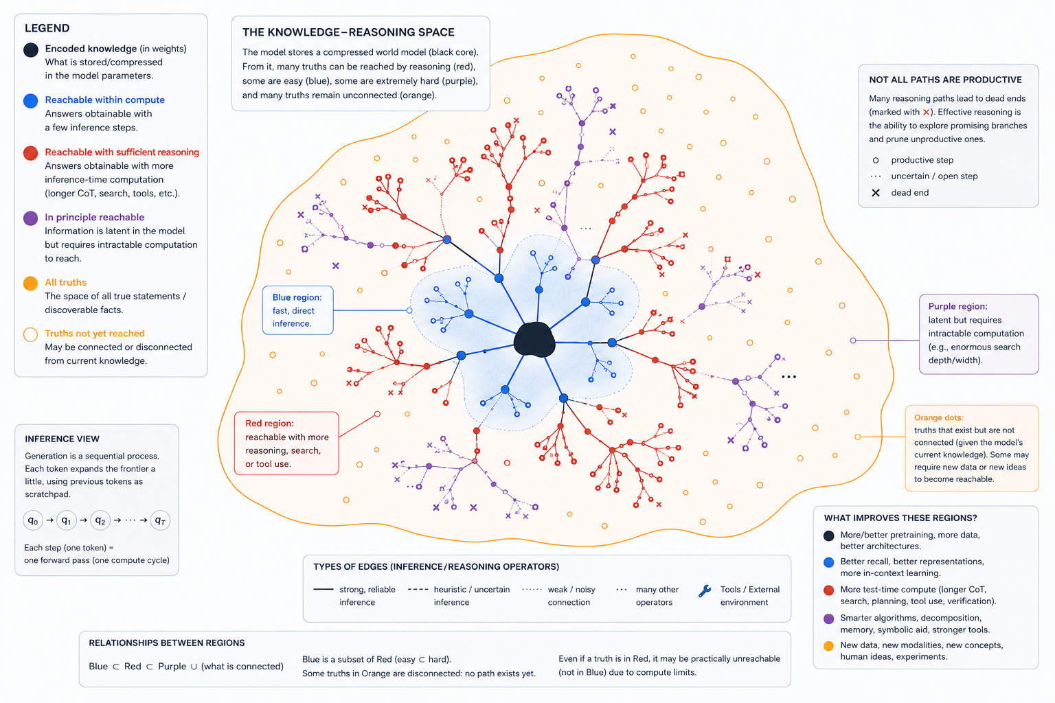
The knowledge-reasoning space. The model stores a compressed world model (the black core). From it, some truths are reachable by cheap inference (blue), more by harder reasoning, search, or tools (red), some are latent but need intractable computation (purple), and many stay unconnected (orange). The regions nest, blue inside red inside purple, and even a truth in red can be out of practical reach when the path to it costs more compute than you have.
Knowledge is not the only budget
There is a second constraint hiding here, and it is the part I find most interesting. A statement can be reachable in principle from what the model knows and still be out of reach in practice, because the path to it is too long. Knowledge and search are different axes. That is the difference between information complexity and computational complexity: asking whether a given chess position is a forced win needs one bit of answer, yes or no, but a staggering amount of computation to produce that bit.
And here autoregression bites hard. The weights are fixed at inference, and the model gets exactly one forward pass per token. There is no way to run ten decompression cycles inside a single token. The only scratchpad it has is the text it has already written, so the true compute budget is not one forward pass, it is the number of generated tokens times the work per pass. This is why chain-of-thought works at all. Letting the model write five hundred tokens of reasoning instead of twenty buys it roughly twenty-five times the computation, and it spends that compute feeding its own partial results back into itself. Chain-of-thought is iterative decompression: unfold a little, read what you wrote, unfold further.
This is the blue region in the figure, sitting inside the red: what is reachable within the compute you can actually spend. The model may know enough to derive a result and still not have the inference budget to walk the path to it, and the figure keeps a separate purple region for the extreme of this, things latent in the weights but needing computation so large they are effectively out of reach. The practical frontier is often not the boundary between the trained and the reachable, but the one between reachable-in-principle and reachable-in-budget. That, I think, is why test-time scaling keeps paying off without touching the weights: chain-of-thought, tree search, self-consistency, tools, none of them add knowledge, they enlarge the blue region inside the red. Pretraining decides what is compressible into the model; inference decides how much of it you can unfold before the budget runs out. Two separate bottlenecks.
Canonical questions, not canonical answers
There is one more idea I cannot let go of. To compress humanity's knowledge well, a model cannot store answers. There are too many of them and they are too redundant. It has to find a small set of latent variables, principles, generators, from which the answers can be rebuilt. I have started thinking of these less as canonical answers and more as canonical questions.
Put some rough numbers on it, because the gap is the whole argument. The largest models are a trillion-ish parameters, a few terabytes of weights once you store them. That already dwarfs things we think of as enormous: all of English Wikipedia is only tens of gigabytes of text. But it is tiny against the full record. Every book humanity has ever written is on the order of a hundred terabytes of raw text, and the web crawls these models train on run into the petabytes. The weights sit one to three orders of magnitude below the material they have to account for. And even if you squeezed all those books down to Shannon's one bit per character, the floor we met earlier, they would still come to ten or twenty terabytes, larger than the model itself. There is no room to keep the answers. The numbers only close if the model throws away the specifics and holds onto the structure that can regenerate them.
A physicist compressing planetary positions does not store the positions, they store Newton's laws and the initial conditions and reconstructs the rest. The real find was the question, "what law generates these observations?", not the table of numbers. Shown $2, 4, 6, 8, 10$, the compressive move is not the list but the hypothesis $x \mapsto 2x$, which stands in for infinitely many lists. A good world model, I suspect, stores far less "the capital of France is Paris" than it stores reusable axes of explanation, cause and effect, optimization, equilibrium, conservation, symmetry, search, recursion, and reconstructs the specific answer on demand.
This loops straight back to where we have been. Entropy, $H(X) = \mathbb{E}[-\log_2 p(X)]$, is uncertainty, and the most powerful way to cut uncertainty across a whole domain is not to memorize its facts but to find the few variables that explain all of them at once. A scientific law is an enormous entropy reducer. It even predicts something we actually observe: models look smartest exactly where the surface data is huge but the generating principles are small and clean, mathematics, physics, code, logic, and shakiest where the knowledge is a pile of arbitrary facts with no compressing structure underneath.
More Than the Objective
“An LLM is a next-token predictor” names the training objective, not the capabilities that can emerge from modeling regularities in data. The open question is how far those learned regularities, combined with inference-time computation, can reach beyond knowledge written in the training set.
Appendix: why random splitting costs $2(\mathcal{H}_n - 1)$
The random-split baseline settles at about 8.4 questions per game, while optimal halving stays near the $\log_2(100) \approx 6.64$ floor. This appendix derives the 8.4 result.
Let $E(N)$ be the average number of yes-or-no questions the random-split strategy needs to pin down a number drawn uniformly from $N$ equally likely candidates. An interval of size one is already solved, so $E(1) = 0$.
Each question picks a split point at random, cutting the $N$ candidates into a left part of size $k$ and a right part of size $N-k$. Because the split point is uniform, $k$ is equally likely to be any of $1, 2, \ldots, N-1$. The secret is uniform over the $N$ candidates, so it falls in the left part with probability $k/N$ and the right part with probability $(N-k)/N$, and it stays uniform inside whichever part it lands in. That gives a recurrence:
Step 1. One question, then recurse into the side holding the secret, averaged over the uniform split point $k$:
That is the orange line in the simulation. Compare it to what an optimal player spends, about 6.7 questions, which can never beat the $\log_2(100) \approx 6.64$ floor: random splitting costs roughly a quarter more for the very same answers. It is not catastrophic, just persistently wasteful, because a random cut is rarely the 50/50 cut that would buy a full bit. As a sanity check, the formula gives $E(2) = 2(\mathcal{H}_2 - 1) = 1$ and $E(3) = 2(\mathcal{H}_3 - 1) = \tfrac{5}{3}$, both of which you can confirm by hand.