Does SDFT Survive the Jump to Mixture-of-Experts?

This post is built with the mathematics as the red thread, and the experiments exist to pin down a quantity the theory has already identified as the thing that matters. We start from why SDFT has a guarantee at all, find an assumption that guarantee leans on, watch that assumption become non-trivial the moment we move to a Mixture-of-Experts, derive a bound that says exactly what would have to be true for the guarantee to fail, and only then go measure whether it is, first up close on one production model where the full apparatus of controls fits, then across six architectures and two domains to learn whether the answer is a property of that model or of the design space.

The guarantee that makes SDFT more than SFT

Start with the method, stripped to its core. SDFT (Shenfeld, Damani, Hübotter & Agrawal, 2026) runs one model two ways on the same query $x$. The student is the policy conditioned only on the query, $\textcolor{#2563eb}{\pi_\theta(y \mid x)}$. The teacher is the same model handed an expert demonstration $c$ in its context, $\textcolor{#7c3aed}{\pi(y \mid x, c)}$. There is no separate teacher network and no external labels: the demonstration is hindsight the model has at training time and will not have at inference, and both policies are the same parameters $\theta$.

(One point of care, which also makes the next derivation exact: the teacher is a stop-gradient target. In practice it is an exponential moving average of the student, still conditioned on $c$; for the derivation what matters is only that we do not backpropagate through it. We treat teacher and student as the same parameters $\theta$ in the forward pass, with the teacher held fixed. The probe later freezes a single checkpoint, so the EMA-versus-live distinction never touches a measurement. Teacher and student are colored purple and blue in the equations below.)

The objective pulls the student toward the teacher through a reverse KL, with the detail that decides everything later: the trajectories are sampled from the student itself.

The $y \sim \pi_\theta$ is the load-bearing detail: the student learns from its own generations, not the teacher's, which is what makes the step on-policy and avoids the compounding errors of off-policy imitation. To see what the objective does to the weights, differentiate it. Because it is a reverse KL over the student's own samples, this is a score-function (REINFORCE) gradient, and it comes out in two short steps.

Two features of this gradient matter for everything downstream. First, the reward is a log-ratio read straight off the policy, no reward model and no labels, just the same network queried with and without the demonstration. Second, it is optimized per token. Worth being precise here, because the exact gradient just derived is the sequence-level one, and inside the product $r(y)\,\nabla_\theta\log\pi_\theta(y)$ sit reward-to-go cross terms: a reward $r_t$ at step $t$ multiplying the score $\nabla_\theta\log\pi_\theta(y_s)$ at every earlier $s$. The future-score terms ($s>t$) vanish in expectation, but the earlier-score terms ($sdetached-trajectory surrogate: sample a trajectory, treat it as fixed, and sum the per-token conditional-KL gradients along it. That drops the state-shift terms, which is standard in on-policy distillation and is the token-level objective the SDFT paper adopts (following Tang and Munos, 2025):

(The paper writes this gradient in its analytic form, summing the log-ratio over the entire vocabulary at each position rather than over the single sampled token. The two are the same gradient in expectation; the single-sample estimator above is the lighter equivalent, and the appendix lists both alongside a Rao-Blackwellized version.)

That log-ratio reward is not an accident of the KL; it is what trust-region RL hands you, and deriving it is what earns the phrase "trust-region step." Start from KL-regularized policy improvement, the same objective that sits under RLHF: the next policy maximizes a reward $r$ while a KL leash to the current checkpoint $\pi_k$ keeps the move local.

This is exactly the log-ratio reward the gradient produced, with the checkpoint $\pi_k$ playing the denominator. At the start of each trust-region step $\pi_\theta = \pi_k$, so the two forms coincide; this is the same old-policy-versus-current-policy bookkeeping that PPO does, if you have seen the Dr.GRPO derivation. The picture is now complete: SDFT is a trust-region RL step in which the unknown optimal policy is supplied for free by the model's own in-context behaviour. No separate model, no labels, the same weights used twice.

The whole reading hinges on one word: local. The step is safe only if the teacher is genuinely close to the student. And at initialization it is, because the two differ by nothing except the conditioning variable:

No parameters have changed; only $c$ has entered the context. So the gap that the trust-region step has to close is exactly the gap that in-context conditioning opens, and nothing more. The question this post asks is what that guarantee is silently relying on.

What "close" is quietly relying on

The trust-region guarantee is a statement about output distributions: monotonic improvement as long as the output-space move stays small, the KL above. It says nothing about parameters or the computational graph, and it does not need to. But a guarantee about the output move is only worth something if the gradient step can realize that move. The step acts on parameters, through a gradient along a particular computational graph, and the question an MoE raises is one of reachability: can a smooth, local parameter step reproduce the teacher's output, or would matching it require a discrete change in which experts fire, the kind of jump a small step cannot make? That is the real content of the word "local," and it is invisible in a dense network.

It is invisible because a dense network is a fixed computational graph. Write the model as $y = f_\theta(\cdot)$: the sequence of operations, and the set of parameters each operation touches, does not depend on the input. Feeding the model $(x,c)$ instead of $x$ changes the activations flowing through the graph, never the graph itself and never which weights participate.

Dense: every output is reachable by a smooth step

A dense forward pass and its backward pass touch the same weights, with 100% overlap. So any output the model produces, including the one it produces when conditioned on $c$, is something the gradient can move toward by smoothly adjusting those very weights. There is no discrete structure to reorganize, so reachability is automatic, and that is exactly why the question never surfaces. The only thing that differs between the teacher and student passes is the activation values.

One honest subtlety on the size of the move, separate from its reachability. How much the output shifts when $c$ enters the context is governed by the smoothness of $f_\theta$ in its input, a Lipschitz property, and standard dot-product self-attention is not globally Lipschitz (Kim et al., 2021); it becomes Lipschitz only on a bounded input domain, which transformers effectively have thanks to LayerNorm and bounded embeddings. So the conditioning move is locally controlled but not globally guaranteed small. That is fine for SDFT, which observes the output KL directly. The load-bearing fact for reachability is the other one: same graph, same weights, so whatever the move is, a smooth step can make it.

So in the dense world the trust-region reading is on solid ground, and the reachability question underneath it is invisible precisely because the answer is always yes. The interesting question is what happens in an architecture where it can be no.

Mixture-of-Experts: the graph stops being fixed

A Mixture-of-Experts layer replaces the single feed-forward block with $E$ separate expert blocks $f_1, \dots, f_E$ and a router. For a token with hidden state $h$, the router emits non-negative gate weights $g_j(h)$, keeps the top $k$, and combines:

The gate $g(h)$ is a function of the hidden state, and the hidden state depends on the context. Put a demonstration $c$ in front of the question and the hidden states change, so the gates can change, so which experts fire can change. The computational graph is no longer fixed by the architecture; it is chosen, per token, by the router, as a function of exactly the variable ($c$) whose effect the trust-region argument is trying to bound.

Before pushing on the worry, it is worth being precise about how independent the experts really are, because the popular mental image (each expert a small disconnected network, routing picking non-overlapping sets) is half right and the other half is what saves us later.

The half that is right: the routed experts genuinely are separate parameter blocks, and per token only $k$ of them fire. The routed-FFN parameters exercised on a given token are a sparse, input-dependent subset, and different conditioning really can exercise non-overlapping subsets. That is the part of the worry with no dense analogue.

The half that is not: the experts do not sit in a vacuum. They ride a shared, always-on backbone: the attention layers, the embeddings, the LayerNorms, the router itself, and crucially the always-on shared expert. In the DeepSeekMoE design (Dai et al., 2024), the shared expert exists precisely so that common computation lives in an always-on path and the routed experts are free to specialize. Those components have identical weights in the teacher and the student pass, no matter what the router does. So the possible non-overlap is confined to the routed-FFN slice, not the whole forward pass.

And the decisive difference from the dense case: there is no architectural guarantee that conditioning leaves routing invariant. Specialization is encouraged by training (load balancing, fine-grained experts, shared-expert isolation; analyzed in Nguyen et al., 2025) but it is an empirical property, not a theorem. The dense assumption that could never be violated is now exactly the thing in question.

Where the gradient goes, and the worst case

To see what a routing change actually does to training, follow the gradient down into a single expert. Expert $j$'s parameters $\theta_j$ enter the layer output $y_t = \sum_{i} g_i(h_t)\, f_i(h_t;\theta_i)$ through exactly one term of the sum, the $i=j$ term, so the chain rule is short:

The gradient to expert $j$ is gated by $g_j(h_t)$. An expert not selected for token $t$ has $g_j(h_t)=0$ and receives no gradient from that token. This is correct sparse credit assignment, and it is the entire reason specialization is possible. Expert $j$'s update is dominated by the tokens where $g_j$ is large, so it learns the subpopulation it is responsible for. The router being informative, that is, $g_j$ being high exactly where expert $j$ is the right tool, is what couples competence to credit.

Now suppose routing is uniform and independent of the input, $g_j(h) = k/E$ for every expert and every token. Substituting:

Two distinct things can break here, and keeping them apart is what makes the next section's axis well-defined.

Failure mode (a): within-model collapse. If a single model routes this way, every $\theta_j$ is pushed toward the same minimizer, the best single feed-forward block on the entire token distribution. The $E$ experts converge to one averaged function, each receiving $k/E$ of the gradient magnitude, and the mixture has the representational diversity of a single expert. This is the routing collapse that load-balancing machinery is built to prevent (Shazeer et al., 2017). But notice: if the teacher and student both route by the same flat $g_j=k/E$, they route identically. There is no teacher-student disagreement, and as the next section makes precise, that is the safe end of the axis. Within-model collapse is a pathology of the model, not of SDFT, so it is not our endpoint.

Failure mode (b): teacher-student disagreement. This is the SDFT-specific one, and it needs care, because the tempting version of the worry is the wrong one. The trajectory is the student's own ($y\sim\pi_\theta$), so the gradient flows through the student's selected experts $g^S$, and those experts genuinely did compute the token. Nothing is miscredited. The teacher's routing $g^T$ enters in exactly one place: the scalar reward $r_t=\log\pi(y_t\mid\cdot,c)-\log\pi_\theta(y_t\mid\cdot)$, how much the demonstration-conditioned model prefers the student's token. The teacher's experts set the magnitude and sign of the signal, not which experts learn. So the real question is not misallocated credit, it is reachability: is that scalar a good target when the two routings differ, that is, can the student's experts, tuned within their own routing, reproduce an output the teacher reached through a different expert subset? When the router is uninformative the two passes select essentially independent subsets (two random draws of 8 out of 64 overlap in about one expert), so the teacher's preferred output is formed through experts the student is not tuning, and reachability is least obvious. Whether the move is reachable anyway is exactly what term (A) measures, and the unreachable extreme is the bad endpoint of the axis we build next.

The bound: damage is linear in routing divergence

Real routing is not uniform, and the dense case is not the only safe point. They are the two ends of a single axis, and we can write the axis down. Take the teacher gates $g^T$ (on the teacher's hidden state $h^T$, which has seen $c$) and the student gates $g^S$ (on $h^S$). Run both over the same token sequence; the gap between the teacher's and the student's layer output, the discrepancy SDFT is working to close, decomposes cleanly:

The decomposition is just an add-and-subtract, the same "insert a clever zero" move that recovers the policy gradient. Insert $\pm\sum_j g^T_j f_j(h^S)$ into $y^T - y^S$ and regroup:

Term (B) is the dense story carried over verbatim: the same experts, evaluated on slightly different activations because the context differs. It is controlled by the experts' local Lipschitz constant times $\lVert h^T - h^S\rVert$, and it is present in any architecture, dense or sparse. Term (A) is the genuinely MoE-specific term, the one with no dense analogue: the gates themselves differ. Bounding it is three standard moves in a row.

That is the result the whole post turns on. The MoE-specific distortion is bounded linearly by the routing divergence, the teacher-versus-student gate disagreement $\lVert g^T-g^S\rVert_1$ (equivalently $2\,\mathrm{TV}$ when the gates form a distribution, the form we use on this model) from failure mode (b). The two endpoints fall right out:

• $\mathrm{TV} = 0$ (teacher and student route identically, whether both sharp or both flat): term (A) vanishes, only the dense-like term (B) survives, and the trust-region guarantee transfers exactly. This is the dense case, recovered.
• $\mathrm{TV}$ maximal (independent routing per pass): the bound opens to $2 F_{\max}$. Hold onto the asymmetry: that is a ceiling the bound permits, not a value term (A) must take. An upper bound binds the safe direction and goes slack in the dangerous one.

So $\mathrm{TV}$ is a one-sided screen, not a verdict. At $\mathrm{TV}=0$ term (A) is exactly zero, and a small $\mathrm{TV}$ bounds it small with no further work, so a small reading genuinely closes the routing question. But a large $\mathrm{TV}$ certifies nothing: the bound only permits a large term (A), it never implies one, and term (A) is in any case a block-level quantity whose effect on the output is a separate propagation question the bound does not touch. A not-small reading therefore says only "now measure term (A) directly, and whether it propagates," which is exactly the second half of this post.

And it is worth being clear about what term (A) is and is not. It is the forward output gap that the routing mismatch opens, $\lVert\sum_j(g^T_j-g^S_j)f_j(h^S)\rVert$, the size of the move the student's experts would have to make to reproduce the teacher's output within their own routing. It is not a story about misallocated gradient: the gradient lands on the student's experts, which is correct, and term (A) is simply how far the reachability question has to travel. Small (A) means the teacher's output is nearly reachable without touching the routing; large (A) means it is not. The bound caps that gap by $2F_{\max}\mathrm{TV}$, one-sided in the same way: small $\mathrm{TV}$ certifies a small gap, large $\mathrm{TV}$ only permits a large one.

The figure has two coordinates and both are measurable, which is better than it sounds, because it means we never have to trust the bound's worst case. The horizontal one, how far routing moves, we read from the gates: the Jaccard overlap of the selected expert sets, and the per-token $\mathrm{TV}$ between the renormalized gate vectors (identical routing gives $\mathrm{TV}=0$). The vertical one, term (A) itself, we need not leave to $2F_{\max}\mathrm{TV}$ at all. The same hooks that expose the gates expose the expert outputs, so $\lVert A\rVert = \lVert\sum_j(g^T_j-g^S_j)f_j(h^S)\rVert$ is directly computable, and the dot's height goes on the plot by measurement.

One honest limit to state up front: this bound is per layer. Showing term (A) small at each of the 27 layers is not the same as a derived end-to-end guarantee on the policy's output; the propagation across layers is something we check empirically, not analytically. So the experiment writes itself in two stages. First, characterize how far routing moves and where (the gate story, next). Then measure term (A) and its dense-like counterpart (B) at the output, directly (the measurement that places the dot's height).

The validation run: L1-16B-A3B up close

Everything from here to the downstream check is one model, in depth. L1-16B-A3B is the validation run: a production MoE on which we can afford the full apparatus of controls, place the operating point on the bound by direct measurement, and rule out the readings that would have broken it. It earns the cross-model screen that follows, where the same decomposition runs on five more architectures with the controls traded for breadth. Read this part as the case that proves the method, not as the whole answer.

The test model is L1-16B-A3B, a medical MoE built on the Gravity-16B-A3B base architecture: a DeepSeek-V3-style design with 16.2B total parameters, about 2.85B active per token, and 27 MoE layers (out of 28 transformer blocks), each carrying 64 routed experts plus one always-on shared expert and a router that keeps the top 8 per token (normalized sigmoid scoring, noaux_tc; attention is the compressed-KV MLA variant). With only about 3B parameters active, "which experts fire and what they compute" is most of the forward pass, so the router is the right place to read $\mathrm{TV}$.

The protocol isolates the one variable in the bound. For each of 200 PubMedQA questions we build two prompts: the teacher prompt (question, a clean DeepSeek-generated chain-of-thought, and the gold-answer line) and the student prompt (bare question). The student greedily decodes a reasoning trajectory. Then we run both teacher and student forward over that exact same token sequence, with forward hooks on every router gate.

That shared-token step is what makes $\mathrm{TV}$ clean. Because both passes route over identical tokens, any difference in the gates cannot come from the tokens; it can only come from the one thing that differs, the demonstration in the teacher's context. Decoding is greedy, so the whole thing is deterministic and reproducible. We run it on the base model and on the same model after SDFT fine-tuning, which lets us ask not only "does the demo move routing" but "does the fine-tuning that the bound is about reorganize it."

At each layer and token we compare teacher and student three ways: JSD (how differently the experts are weighted, in bits), Jaccard (whether the same experts fire, the direct overlap), and eff-N ($1/\sum_i w_i^2$, how concentrated the weighting is). These three live in routing space: they see which experts are chosen, not what those experts compute. They answer "how far does routing move, and where," which is the horizontal axis of the bound. Turning that into the vertical axis, how much the routing shift actually perturbs the output, takes the expert outputs themselves, which we bring in for the direct measurement of terms (A) and (B) at the end.

The global divergence, and what the bound says about it

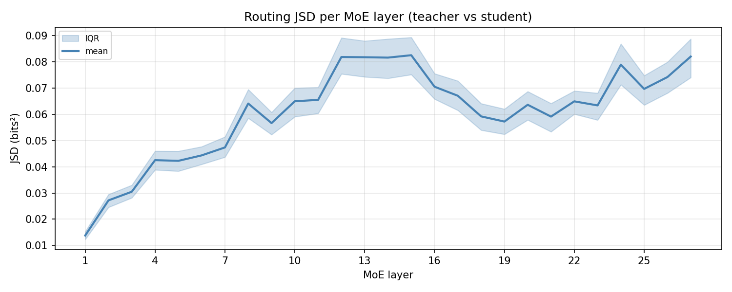
Averaged over all 27 layers and all generated tokens, routing barely moves: JSD about 0.045 bits (the maximum is 1.0), Jaccard about 0.87 (roughly 7.5 of 8 experts shared), eff-N shift about 0. Through the bound, a routing divergence this small caps the worst case for term (A): the mismatch can contribute only a little to the output gap, and the trust-region picture looks intact at the gate level. Whether term (A) is actually that small, rather than merely bounded by it, is what the direct measurement settles later. The structure is also stable across depth: divergence peaks at Layer 15, with a characteristic rise, dip, rise shape.

The cross-checkpoint comparison is the one that speaks directly to the bound. SDFT improves the bare student substantially, and changes the teacher-to-student routing gap by almost nothing:

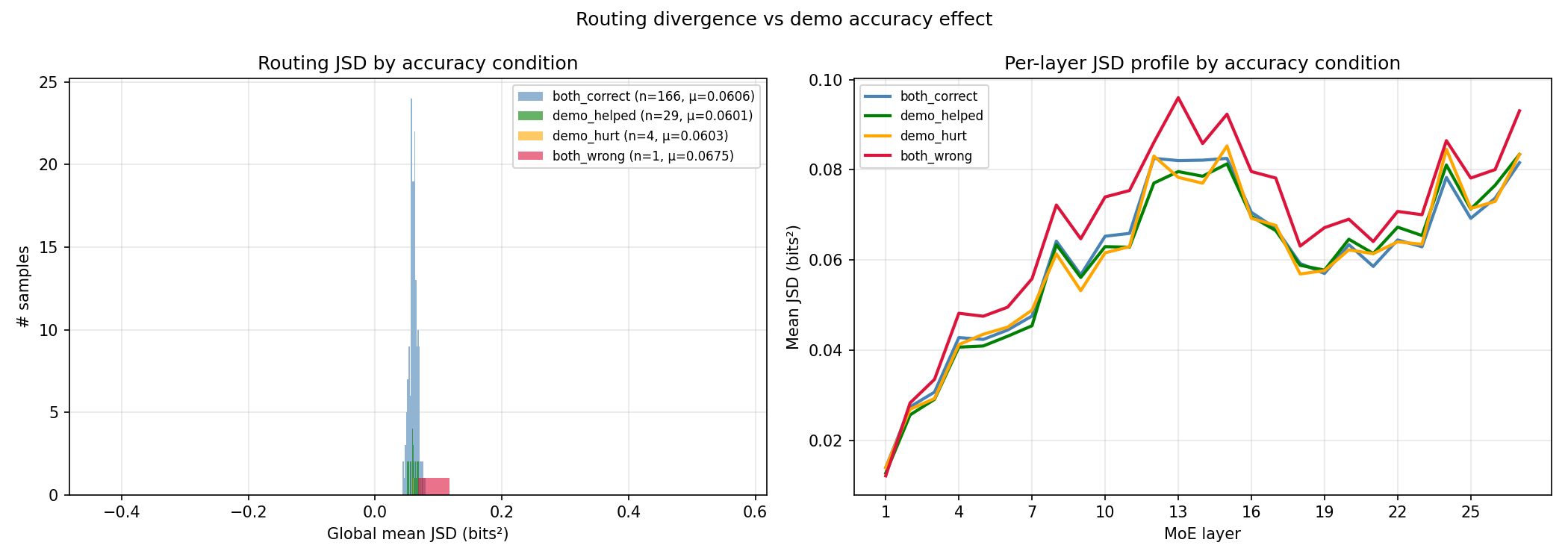
Accuracy moves by $+8.5$ points; the routing gap barely moves with it, the expert overlap (Jaccard) shifting by $+0.003$ and the peak layer not at all. Whatever SDFT improved, it did not improve it by reorganizing which experts fire. And the routing gap does not even track correctness: split the samples by accuracy outcome and the JSD is flat across all of them.

A dissociation the bound predicts is benign

Large behavioral change from the demonstration; near-zero change in expert routing; routing that does not even correlate with accuracy. In the language of the bound, $\mathrm{TV}$ is small and SDFT does not grow it, so term (A)'s worst case is small and the gain is happening at the generation level, not the routing level. That is the gate-level read; the direct measurement of term (A) at the output will confirm it and sharpen the reason.

This is where a less careful reading would stop. It should not, for one reason that is statistical and one that is interpretive. The statistical reason: a Jaccard of 0.874 can be read two ways. "Roughly 7.5 of 8 experts shared, essentially the same routing," or, just as truthfully, "about 55% of tokens swap at least one expert, routing is meaningfully shifted." Same number, opposite spin, and a global mean cannot say which is honest. The interpretive reason is sharper: a mean over 27 layers and hundreds of tokens is exactly the statistic that can dilute a real, concentrated effect to nothing. The bound is about $\mathrm{TV}$ token by token, not on average. So before trusting the small number, we have to ask where the divergence lives.

Where the divergence actually lives

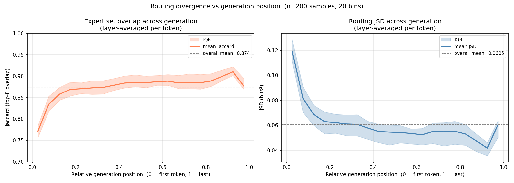
Break $\mathrm{TV}$ out by token position and the flat 0.045 turns out to hide a sharp transient. The first generated token, the <think> token that opens the reasoning, diverges about six times the body, then decays to the plateau within a handful of tokens. There is a smaller bump at the very end.

The qualitative texture matches a clean story. Read the openings and the divergence has an obvious source:

• Start zone, high divergence. The teacher opens straight on the topic ("The study examines whether...") while the student opens with deliberative scaffolding ("Okay, let's tackle this question..."). Different first tokens recruit different experts from token one.
• Body, low divergence. Both models do the same job: read the abstract, weigh the evidence. The shared task recruits the same experts.
• End zone, a bump. The teacher closes with </think> and a bare letter; the student often uses a markdown answer format. Different token types, different experts.

It is tempting to take the spike at face value: the demonstration steers how the reasoning opens, and after that the two converge. But the bound demands a more careful question, because a spike at the opening is partly guaranteed by the setup, independent of anything the demonstration says.

The trap baked into the first token

At the first generated token, the teacher has just consumed an entire demonstration and the student has consumed nothing. Their contexts are maximally different right there, and most similar later. So a divergence spike at token 0 is partly mechanically guaranteed: it is what any long prefix would produce, regardless of content. "The spike exists" is not yet a finding. The question the bound actually cares about is whether the spike is term (A) driven by the demonstration's content, or a benign effect of a demonstration merely being present.

This distinction is the whole game. A content-driven spike, the demonstration recruiting specific reasoning experts, is exactly the "different computational path" that makes term (A) real and dangerous. A presence-driven spike, routing merely registering that a long context arrived, inflates the raw $\mathrm{TV}$ number without corresponding to any specialized re-routing, and is harmless to the guarantee. You cannot tell them apart by looking at the spike. You separate them with controls.

Content or presence: three controls

Control 1: is the spike even above the noise floor?

0.29 is meaningless without a scale. Under greedy decoding, rerun-to-rerun variance is exactly zero, which is the wrong floor. The right floor is how much routing moves for unrelated content at all. So we measure three quantities at the opening token on equal footing: S, the demo-teacher against its own bare student; N, two bare students on different questions; and F, the demo-teacher against some other question's student.

Two readings, pointing opposite ways. The encouraging one: S (0.29) sits far above N (0.13), so the spike is real, not a decoding artifact. The unsettling one: F is about equal to S. If the demonstration's effect were specific to this question, the teacher would route more like its own student than like a random other one. It does not; the teacher's opening routing is equidistant from everybody. That is the signature of presence, not content. The next control settles it.

Control 2: the length-matched irrelevant demonstration

Here is the control the bound is really asking for. For each question, build a second teacher prompt with the same question, the same gold-answer hint, and the same length, but with the worked example replaced by the chain-of-thought of a completely unrelated question (length-matched to a fraction of a percent, otherwise presence is confounded with length). If the spike is content, an irrelevant demonstration should produce far less divergence. If it is presence, it should reproduce almost all of it.

The spike is presence, not content

An unrelated demonstration reproduces 97% of the spike, and Control 1's F-about-equal-to-S said the same thing from another angle. The opening divergence is context arrival, not the demonstration recruiting special reasoning experts. For the bound this is the better news: the raw $\mathrm{TV}$ at the opening overstates term (A), because almost all of it is presence that does not correspond to a content-driven change of computational path. The expert path is shared, not content-reorganized.

Control 3: split the block output into routing and context

The MoE block adds the routed output $h_{\text{routed}}$ and the always-on shared expert's output $h_{\text{shared}}$. The shared expert is a clean probe: identical weights in both passes, so the only way its output can differ is if attention fed it a different summary of the context. Reading the divergence of each, both diverge by about the same amount at the opening, roughly two standard deviations, and the output distribution there barely moves.

It is worth seeing why that is the expected result, not a failed localization, because the reason is exactly the decomposition from Section 5. The routed output's teacher-student divergence is itself $(\mathrm{A}) + (\mathrm{B}\text{ through the routed experts})$: the router shift and the context shift carried through the experts. The shared output's divergence is $(\mathrm{B}\text{ through the shared expert})$. Both diverging by the same amount is precisely what "term (A) is small, the effect is the context shift (B) flowing through both paths" predicts. So Control 3 does not fail to localize; it isolates term (A) from term (B) and says the routing piece is not where the action is.

Two threads remain. One is the 2.6% content sliver that survived Control 2: small as it is, does it predict when the demonstration actually helps? The other is the bound's vertical axis itself, term (A) measured directly rather than bounded. We take the content sliver first, because it carries the sharpest methodological caution in the study.

The residual content effect, and a confound that tracks the outcome

The 2.6% content effect is real, and it would be a satisfying ending if that sliver were what carries the demonstration's accuracy benefit. To test it, define a per-question content increment that subtracts the presence component out:

Measured over the reasoning body (the opening's output is inert, so if content acts anywhere it is where answers are produced), the question is whether a sample's $\Delta_i$ predicts that the demonstration helped, that is, turned a wrong student into a right teacher.

It does not survive scrutiny, and the reason is structural. Look at how "helped" is defined: helped = teacher_correct AND NOT student_correct. A helped sample is, by definition, one where the student was wrong. And $\Delta_i$ is built from a JSD whose second argument is the student's routing, which moves with whether the student reasoned correctly. The outcome label is sitting on one side of the metric. "Helped" may simply be "student was wrong" in a better outfit.

The "helped vs not-helped" gap is $+0.00218$; the "student-wrong vs student-right" gap is $+0.00216$. The ratio is 1.01: the same effect. The clean test seals it. Within the student-wrong questions only, holding correctness fixed, demonstration-helping moves the increment not at all ($p = 0.68$). Controlling for the confound, helping adds about 0.4% of the variance. Nothing.

What does survive is small and points the safe way. Beyond presence, a relevant demonstration makes the teacher route more like the bare student, not less: a 3.7% body convergence ($p = 2.7\times10^{-16}$), while an irrelevant demonstration pushes routing apart. In the language of the bound, the residual content effect reduces $\mathrm{TV}(g^T,g^S)$ rather than growing it. A good demonstration nudges the teacher onto the student's expert path, which is exactly the direction an on-policy interpretation wants. Even the leftover signal points toward shared computation.

What the bound says, now that term (A) is measured

The gate story fixed the dot's horizontal coordinate. Routing barely moves (true-weight $\mathrm{TV}\approx0.17$ in the reasoning body), the movement is mostly context presence rather than content, and the residual content effect is convergent. But the bound has two factors, $2F_{\max}\mathrm{TV}$, and the gates pin down only $\mathrm{TV}$. Reading the dot's height off the bound would mean trusting an unmeasured $F_{\max}$. We do not have to. The same hooks that expose the gates expose the expert outputs, so term (A) is directly computable with the model's true routing weights, per token and per layer, over all 200 samples:

Term (A) is not vanishing, but it is small in the norm that propagates. Against the MoE block's own output it is a 9.7% perturbation; against the residual stream it is added to, the quantity that actually reaches the logits, it is 4.4% per layer. That residual-relative number is the one that answers the worry, and it is small with no further argument. The earlier $2F_{\max}\mathrm{TV}$ reading was not wrong, only uninformative: it never measured $F_{\max}$. Measured, $F_{\max}\approx0.99\,\lVert y\rVert$: the block output is no larger than its single dominant expert. With that, the bound $\lVert A\rVert\le2F_{\max}\mathrm{TV}$ holds at every one of the 3.1 million layer-token instances, confirming that $\mathrm{TV}$, $\lVert A\rVert$, and $F_{\max}$ are consistently defined on the same gates, but its median tightness is only $0.30$ and its maximum $0.67$. The bound is real and about three times loose, so reading the dot's height off it would have overstated term (A) roughly threefold. The dot sits at about 30% of the ceiling, by measurement, which is the whole reason measuring term (A) directly earned its keep.

And term (A) is the minority term. Its sibling (B), the context-shift carried through the teacher's selected experts, is 9.5% of the residual, about $2.2\times$ larger, and the two reconstruct the full routed difference to better than 1% per token (an implementation cross-check, since $A+B=\Delta_{\text{routed}}$ is an algebraic identity). It is "dense-like" in the sense that matters here, it is the MoE analogue of the input-conditioning a dense model would show, the same experts on a shifted context, rather than a change in which experts fire. The teacher-student difference is carried by that term, not by the MoE-specific routing term.

And the output closeness, not term (A), is what actually carries the guarantee. The most direct evidence that the step is local is the teacher-student output KL over the same tokens, median 0.003 nats. If the two output distributions are that close, the step is a small output-space move regardless of the routing underneath, which is exactly what the trust-region argument requires. Terms (A) and (B) are the composition of that closeness, the account of why it is dense-dominated, not the evidence for it. The verdict rests on the measured closeness; the decomposition explains its shape.

That closeness is tail-concentrated, and the concentration is the mechanism behind the headline dissociation. The median body output KL is 0.003 nats but the mean is 0.30, with the top 1% of tokens carrying a quarter of the mass: most tokens barely move while a handful of pivotal ones do the work, which is how a large accuracy gain coexists with a near-zero typical-token change. And per-layer 4.4% routing nudges do not accumulate into a meaningful output shift across the 27 layers, the empirical statement that the per-layer bound does not compound.

Even where divergence concentrates, routing mismatch is a minor part of a minor part. On the most divergent 1% of tokens, term (A) and term (B) co-vary strongly ($+0.78$), so the question is what (A) explains beyond the dense-like (B). Isolating it (the semipartial $\Delta R^2$ of $\lVert A\rVert$ given $\lVert B\rVert$ and $\lVert y\rVert$), routing mismatch adds only 1 to 2% of unique variance to the output divergence (1% at the top 1% of tokens, rising to 2% at the top 5%), against about 2.5% for (B), a partial $f^2 \approx 0.012$ that sits below the conventional threshold for a small effect and reads as nonzero only because $n$ is large. And the full routed path explains just a fifth to a quarter of even the tail divergence; the rest lives downstream in attention, the shared expert, and the unembedding, exactly where Control 3 pointed.

The routed-path decomposition is now measured, not inferred by elimination: (A) and (B) are both quantities on the table, and (A) is the smaller. The first boundary is that the majority of the tail output divergence stays unlocalized: the routed path explains under a quarter of it, so the remainder is attributed to attention, the shared expert, and the unembedding by elimination, not measured there. That inference is the harmless kind, because the load-bearing claim is the negative one, not in routing, and that is measured directly. The second boundary is scope: one MoE, one dataset, and $n=200$ for the routing probe, so the verdict here is stated for this model, not for Mixture-of-Experts in general, which is exactly the gap the cross-model screen closes below. The third is temporal: this is the per-step question, whether a single trust-region step is realized. The practically loaded question for MoE-SDFT is multi-step, whether the slightly mismatched detached-trajectory gradient drifts routing or load balance over thousands of steps. The base-versus-checkpoint-2000 comparison (routing topology stable, peak layer unchanged) is one reassuring point on that trajectory, not the trajectory itself, and the multi-step dynamics are the subject of the closing section. The off-policy risk worth monitoring in training is likewise not routing but the start-zone style: the demo-anchored direct opening could push the fine-tuned model to state conclusions early even without a demonstration at inference, a generation-level effect that lives in term (B), not (A).

Does the theory's prediction hold downstream?

The bound, plus the measurements, says SDFT's benefit is a generation-level effect rather than a different expert path. If that is right, the benefit should at least not behave like benchmark overfitting: improving the trained tasks should not come at the cost of everything else. The downstream check is the full post-training run that produces L1-16B-A3B, evaluated both on the datasets SDFT trained on (in-domain) and on a battery of held-out medical benchmarks it never saw. SDFT was run in three data configurations that differ only in how the multi-turn HealthBench data is handled.

Shaded columns are in-domain (the datasets SDFT trained on); the rest are held out. SDFT configs: (1) HealthBench dropped, (2) HealthBench multi-turn flattened, (3) HealthBench last-turn only. Config (3) is strongest overall; config (1) regresses HealthBench exactly because it stopped training on it.

There are two possible baselines here, and they tell completely different stories. The gap between them is the same confound lesson as before, one more time. Averaging the columns:

• SFT on the benchmark data only nails the three target benchmarks (in-domain average about 89) and falls off a cliff everywhere else (held-out average about 44). Classic overfitting.
• SFT on all the data lifts the held-out average to about 60, but gives up the in-domain peak (in-domain average about 82).
• SFT all, then SDFT (config 3) recovers most of the in-domain peak (back to about 87, near the benchmark-only model) while holding the held-out average where all-data SFT left it (about 60).

The only pair that isolates SDFT is SFT-all versus SFT-all-plus-SDFT: in-domain rises about 5 points and held-out stays essentially flat. One caveat keeps even that honest: the pair isolates the SDFT step cleanly only insofar as the HealthBench handling matches across the two arms; where the config changes it (config 3 keeps last-turn only), a sliver of the in-domain $+5$ is the data choice rather than SDFT. With that noted, the honest statement is the narrow one: SDFT gives back the in-domain sharpness that broad SFT trades away, without re-introducing the overfitting that benchmark-only SFT suffers from. No generalization tax. Flat held-out does not show the skill transfers to new tasks, a skill that travelled would have lifted held-out and it did not, but it does show the in-domain gain is not bought by sacrificing generalization. That is the consistent reading with the routing story: a generation-level effect, not a benchmark memorized through a special expert path.

The screen: every architecture, both domains

L1 is one model, and one model cannot tell you whether the verdict is structural or a lucky property of this design: one shared expert, sigmoid gating, 64 experts with 8 selected. The bound is a product, $F_{\max}\lVert g^T-g^S\rVert_1$, and different architectures push on its two factors in opposite ways. So we run the same decomposition on five more architectures chosen to span the axes the bound says matter, and on a second domain, holding the machinery fixed and trading the L1 controls for breadth.

Six MoEs spanning 8 to 128 experts, shared and shared-free, sigmoid and softmax, and gates that sum to anywhere from 0.36 to 2.45. gpt-oss is routing-only (its quantized experts fail the term-(A) reconstruction gate), so it contributes routing metrics but not a term-(A) point.

Two relative metrics carry the rest of the post, and keeping them apart is the whole game. relA/res $=\lVert A\rVert/\lVert\text{residual}\rVert$ is the safety verdict: term (A) as a fraction of the norm that actually propagates to the logits, the number that rates a model safe. But it is confounded across models by how heavily each architecture weights its routed path into the residual ($\Sigma g$ spans sixfold), so it is a per-model verdict, not a clean cross-model quantity. relA/block $=\lVert A\rVert/\lVert y_{\text{block}}\rVert$ divides that weighting out, numerator and denominator both scaling with the gates, so it is the $\Sigma g$-invariant number, comparable across architectures. We report both, and they say different things on purpose.

Read the bands, not the rows. Across all five architectures that yield a term (A), and both domains, relA/res lands between 1.9% and 6.1%, relA/block between 9.0% and 13.9%, and Jaccard between 0.82 and 0.91. Every architecture, every domain: the routing-mismatch term is a single-digit-percent perturbation of the propagating residual, and 82 to 91% of the selected experts are identical in the teacher and student passes. The mismatch is mostly a gate-reweighting of largely the same experts, not a wholesale swap. The L1 verdict was not a property of L1: SDFT survives across coarse and fine routing, shared and shared-free, sigmoid and softmax, and stochastic, sub-stochastic, and scaled gating alike.

The two shared-free corners are worth a sentence each, because they sit on the bound's two factors. Mixtral (8/2) is the $F_{\max}$ corner: flipping one of two selected experts moves half the routed compute, so $F_{\max}$ is large. It came out among the safest of the set (relA/res 0.022, just behind Qwen3's 0.019), because coarse routing barely moves ($\lVert\Delta g\rVert_1$ small) and the product is what matters. Qwen3 and OLMoE are the routing-distance corner: fine-grained, shared-free, two top-8-of-128-or-64 draws that overlap less and respond more to content. They show the largest routing distance in the set, and they still survive. Neither corner breaks.

Why the margin holds: the backbone, not the router

The screen says SDFT survives. The stronger result is the reason, and it is sitting in the gap between the two metrics. relA/block, the cross-model mechanism number, holds a tight 1.5× band (0.090 to 0.133 on PubMedQA). relA/res, the safety number, spans $\sim$3× (0.019 to 0.056). Since relA/res $=$ relA/block $\times$ (block/residual), and relA/block is nearly constant across the set, the entire $\sim$3× spread in safety is set by block/residual: how much of the residual stream the MoE block owns, versus the always-on paths. The routing-mismatch magnitude is similar everywhere; what differs is how much it is diluted on the way to the logits.

And the ranking confirms it: the relA/res order is the block/residual order, identically, in both domains.

PubMedQA; block/residual $=$ relA/res $\div$ relA/block. The relA/res ranking is the block/residual ranking. relA/block does not order the column.

The cleanest read is Qwen3 versus OLMoE. Their relA/block is comparable, both inside the tight band (0.133 vs 0.124), and the safer model, Qwen3, if anything carries the slightly larger routed-block mismatch. Their relA/res is opposite (0.019 vs 0.056), because the MoE block is about 14% of Qwen3's residual and about 45% of OLMoE's. Comparable routing mismatch, a $\sim$3× difference in safety, set by how much of the residual the always-on backbone owns. That inverts the lazy reading: the safe model has more routing movement, so safety cannot be a routing property. For a pair with truly equal routed-block mismatch, take Mixtral and L1 (relA/block 0.094 and 0.098): L1's relA/res is double Mixtral's (0.044 vs 0.022) because its block owns double the residual (0.45 vs 0.23), the same mismatch diluted half as much.

This is the single-model finding made general. On L1 the visible backbone was the shared expert: term (B), the dense-like context-shift, ran about $2.2\times$ term (A), and the shared expert carried about half the residual. The screen shows the idea is larger than the shared expert. Even the shared-free models have an always-on backbone, attention, embeddings, and the LayerNorms, identical in both passes, and the same dilution holds. "Term (B) is the backbone" generalizes to "the always-on contribution is the backbone." The routing mismatch is small in the routed block, and then everything that runs for every token dilutes it into the residual. The dilution sets the margin.

The per-layer picture: where the exposure lives

The headline relA/res is an average over layers, and an average can hide its own shape. Plot the magnitude-weighted relA/res at every MoE layer against normalized depth, input to output, and the shape is consistent across the screen: exposure is low at the entry, rises to a mid-stack hump where the routed path carries the most of the residual, and lifts again into a spike at the final layer. The load-bearing fact is the ceiling. Across all five models and both domains, no single layer's relA/res exceeds about 11% (OLMoE's output layer, the highest point anywhere). The bound holds layer by layer, not merely on the pooled average, which is the stronger statement.

The terminal spike is the one to look at, because it sits exactly where a routing blow-up would show up, and it is not one. Decompose the final layer the way the screen does, relA/res = relA/block × block/res, and in every case the spike is dilution-dominant, block/res driven: the always-on backbone contributes less of the residual near the output, so the same routed mismatch lands on a smaller denominator. In seven of the ten model-domain cases it is pure, with relA/block flat or at a local minimum (it actually falls at the output, an uptick below 1); for L1, Qwen3, and DeepSeek-V2 relA/block drops to its minimum exactly where relA/res peaks, dilution in its purest form. The other three, OLMoE on both domains and Mixtral on math, add a small routing uptick on top (relA/block 1.06 to 1.21× its preceding three layers), so they read as dilution-dominant with a minor routing contribution.

The final MoE layer of each model. An uptick below 1 means relA/block fell at the output (the spike is pure backbone-thinning); above 1 means a small routing contribution rode along.

One honest counter-note rides on that last layer. Math sharpens the spike, and we can measure which branch does it. For Mixtral, OLMoE, and DeepSeek-V2 the final-layer relA/block grows from PubMedQA to GSM8K while block/res barely moves or falls, so the extra sharpening is the routing branch, not more dilution; only L1 sharpens through block/res. So the broad story, that routing is content-blind, holds with one localized exception: at the very last layer the gate disagrees a little more on math than on medicine. The likely reason, a tighter and more format-constrained output distribution, is a hypothesis rather than a measurement, so state it honestly as a measured factor with an open cause.

Three textures the screen leaves behind

Granularity. Hold shared-status and gate convention fixed (the no-shared softmax models) and let only granularity move: relA/block rises cleanly with it, Mixtral 8/2 (0.110) $<$ OLMoE 64/8 (0.122) $<$ Qwen3 128/8 (0.139) on GSM8K, monotone. Finer routers respond more to content and move more per token, so the thin-margin corner of the design space is fine-grained and shared-free. It still survives; it is just where the backbone has the least to dilute with.

Dilution, not absorption. The shared expert dilutes the routing mismatch, it does not actively cancel it, and the distinction is one the data can defend. The numerator $\lVert A\rVert$ is the same whether we divide by the block output (relA/block) or by the routed output alone (relA/routed); the rise when the shared expert leaves the denominator (L1 0.098 $\to$ 0.126, DSv2 0.090 $\to$ 0.145) is purely the residual shrinking, the shared expert's share of the backbone (shared_frac 0.54 on L1, 0.65 on DSv2). That shows the shared expert is a large residual backbone, the term-(B) story, not that it reaches in and absorbs the mismatch, which would be a stronger causal claim a denominator decomposition cannot make. We claim the weaker, clean thing.

Cross-domain. Math runs a little hotter than medicine. From PubMedQA to GSM8K the relA/block band shifts up (floor 0.090 $\to$ 0.102, ceiling 0.133 $\to$ 0.139) with its width roughly preserved, slightly narrower (0.043 $\to$ 0.037). The band moves up as a whole, spread intact, not a convergence: most architectures perturb slightly more on harder reasoning, with OLMoE the lone exception (it edges down, 0.124 $\to$ 0.122), and the ranking survives the move. The honest report is a range, math $\gtrsim$ medical, not a single number.

What this does not show: the trajectory

One honest boundary contains everything above. Every number here, on L1 and across the screen, is per-step: a snapshot of the trust region at a frozen checkpoint, teacher and student passes compared on identical tokens at a single moment. It establishes that one trust-region step is realized, that the output move the demonstration opens is reachable without a routing change a small step cannot make. It does not establish what happens when you take thousands of steps.

The gap is exactly the one the derivation flagged: SDFT optimizes the detached-trajectory surrogate, which drops the state-shift terms, and the open question is whether the small per-step routing mismatch compounds over a full run, or whether load balance drifts as the router is trained. The base-versus-checkpoint-2000 comparison on L1 (routing topology stable, peak layer unchanged after 2000 steps) is one reassuring point on that trajectory, not the trajectory itself. The multi-step study, which brackets the shared-expert axis with L1 (shared) at one end and the shared-free OLMoE at the other, tracking routing drift and load-balance collapse across checkpoints, is in progress. Until it lands, the scope is precise: the per-step trust region survives the jump to Mixture-of-Experts, across the design space, and the structural reason is the always-on backbone. Whether the trajectory does is the next question.

The bound was the whole argument

Look back at what carried the weight. The trust-region guarantee is output-space, and the only question was whether a smooth step can realize the output move, automatic in a dense graph and not obviously so in an MoE, where matching the teacher might demand a routing change a small step cannot make. Turning that reachability question into the decomposition $y^T - y^S = (\mathrm{A}) + (\mathrm{B})$ and the bound $\lVert A\rVert \le F_{\max}\,\lVert g^T - g^S\rVert_1$ collapsed it into one measurable term, (A), with the dense case and maximal routing disagreement as its two endpoints. After that there was nothing left to argue in the abstract; the work was to measure where reality sits, first up close on one model, then across the design space.

The measurements put the operating point near the safe end and held it there, on every architecture and both domains. Routing barely moves (Jaccard 0.82 to 0.91), term (A) is a 2 to 6% perturbation of the residual that propagates, and the gap is carried by the dense-like term (B) a dense model already carries. And the screen handed back something a single model could not: the reason. The safety margin is not routing happening to be stable; it is the always-on backbone diluting a small routing mismatch, and the spread across architectures tracks how much of the residual that backbone owns. Where a model has more always-on path, attention plus a shared expert, term (A) is diluted more, and the margin is larger. On L1, the controls that would have broken the verdict all failed; across the screen, the verdict held everywhere and came with a mechanism.

Appendix

Single-model deep dive (L1-16B-A3B, PubMedQA, n = 200).

Cross-model screen (five term-(A) models, n = 200 per model per domain).

Routing extraction, metrics, the gate analysis (the three controls), and the direct term-(A) and term-(B) decomposition at the block output, plus the per-test reports, live in the project repository. All term-(A)/term-(B) figures are measured with the model's true realized routing weights over n = 200 (about 116k body tokens); the reconstruction $A+B=\Delta_{\text{routed}}$ is an algebraic identity used only as an implementation check, and the tail regressions control the $+0.78$ collinearity between $\lVert A\rVert$ and $\lVert B\rVert$. Figures: per-layer JSD and accuracy-split from the base-model run; positional divergence from both checkpoints. Downstream evaluations come from the full post-training pipeline, a separate set of runs from the controlled PubMedQA routing probe. The cross-model screen runs the same decomposition through a per-architecture RouterSpec (gate convention and shared-expert handling verified empirically from a forward pass, not read off configs), forms term (A) on each model's true realized gates via the $\ell_1$ bound, and requires the per-model reconstruction $A+B=\Delta_{\text{routed}}$ to close to under 1% before a model's term (A) enters the tables; gpt-oss is held routing-only because its mxfp4 experts fail that gate. The multi-step study referenced in the closing section is in progress and not reported here.

References

1. Shenfeld, I., Damani, M., Hübotter, J., Agrawal, P. (2026). Self-Distillation Enables Continual Learning. arXiv:2601.19897
2. Kim, H., Papamakarios, G., Mnih, A. (2021). The Lipschitz Constant of Self-Attention. ICML 2021. arXiv:2006.04710
3. Shazeer, N. et al. (2017). Outrageously Large Neural Networks: The Sparsely-Gated Mixture-of-Experts Layer. ICLR 2017. arXiv:1701.06538
4. Dai, D. et al. (2024). DeepSeekMoE: Towards Ultimate Expert Specialization in Mixture-of-Experts Language Models. arXiv:2401.06066
5. Nguyen, H., Doan, T. T., Pham, Q., Bui, N. D. Q., Ho, N., Rinaldo, A. (2025). On DeepSeekMoE: Statistical Benefits of Shared Experts and Normalized Sigmoid Gating. arXiv:2505.10860.
6. DeepSeek-AI (2024). DeepSeek-V3 Technical Report. arXiv:2412.19437
7. Tang, Y. & Munos, R. (2025). On a few pitfalls in KL divergence gradient estimation for RL. arXiv:2506.09477

Models screened.

8. Jiang, A. Q. et al. (2024). Mixtral of Experts. arXiv:2401.04088
9. Muennighoff, N. et al. (2024). OLMoE: Open Mixture-of-Experts Language Models. arXiv:2409.02060
10. DeepSeek-AI (2024). DeepSeek-V2: A Strong, Economical, and Efficient Mixture-of-Experts Language Model. arXiv:2405.04434
11. Yang, A. et al. (Qwen Team, 2025). Qwen3 Technical Report. arXiv:2505.09388
12. OpenAI (2025). gpt-oss-120b & gpt-oss-20b Model Card. arXiv:2508.10925