Picture yourself standing before an enormous pipe organ with a million stops, each one controlling the pitch and volume of a different pipe. Your task? To create a perfect symphony from chaos. After your first attempt produces nothing but cacophony, you face the fundamental challenge: which stops should you adjust, by how much, and in what direction?
This is precisely the predicament faced by every neural network during training. Each weight and bias is like one of those organ stops, and the network must learn to "tune" millions of parameters simultaneously to minimize prediction error. The breakthrough that made this possible wasn't just clever engineering—it was a profound mathematical insight that transformed machine learning forever.
Welcome to backpropagation: the algorithm that taught machines how to learn from their mistakes with mathematical precision.
The Calculus of Blame
At its mathematical core, backpropagation is an application of the chain rule from calculus, but thinking of it merely as "fancy derivatives" misses its elegant conceptual beauty. The algorithm embodies a systematic approach to credit assignment—it traces the path of influence from output error back through the network's computational graph, quantifying exactly how each parameter contributed to the final mistake.
🔍 The Key Insight
The gradient of the loss function with respect to any parameter tells us the instantaneous rate of change of error with respect to that parameter. In other words: "If I nudge this weight by a tiny amount, how much will my error increase or decrease?" This is the information we need to improve our model systematically.
The genius lies in the recursive structure: to compute how a parameter in layer $\ell$ affects the final loss, we need to know how the outputs of layer $\ell$ affect the loss. But that's exactly what we computed for layer $\ell+1$! This creates a natural backward flow of gradient information, hence "back-propagation."
Mathematical Foundations
The Chain Rule
Before diving into neural networks, let's establish our mathematical foundation. The multivariate chain rule states that for a composite function $f(g(x))$:
This is the mathematical engine that powers backpropagation. A neural network is essentially a deeply nested composite function, and the chain rule allows us to efficiently compute gradients by decomposing the problem into manageable pieces.
Activation Functions and Their Derivatives
Before we can derive backpropagation, we need to understand the building blocks. Let's rigorously derive the derivatives of common activation functions.
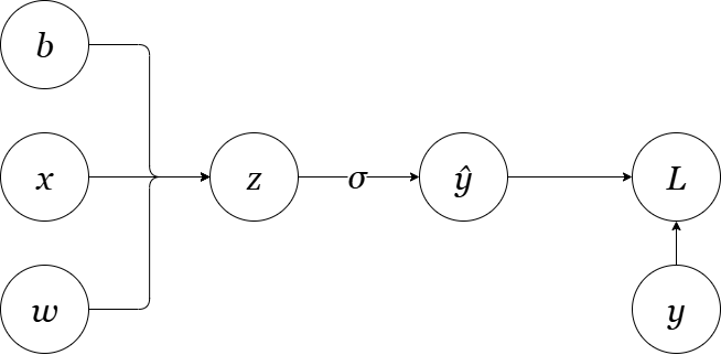
The Sigmoid Function
The sigmoid function provides a smooth, differentiable way to squash any real number into the range $(0,1)$:
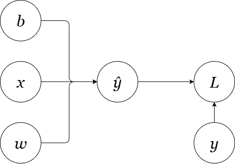
Let's start with the simplest case and build our intuition step by step. Consider a single linear neuron with one input:
Figure 1: A simple linear neuron transforming an input 'x'.
Note: We multiply by 1/2 for mathematical convenience. It simplifies the derivative during backpropagation, as the '2' from the power rule cancels out, leaving a clean error term.
Forward Pass
Step 1: Linear transformation: $\hat{y} = wx + b$
Step 2: Loss computation: $\mathcal{L} = \frac{1}{2}(y - \hat{y})^2$
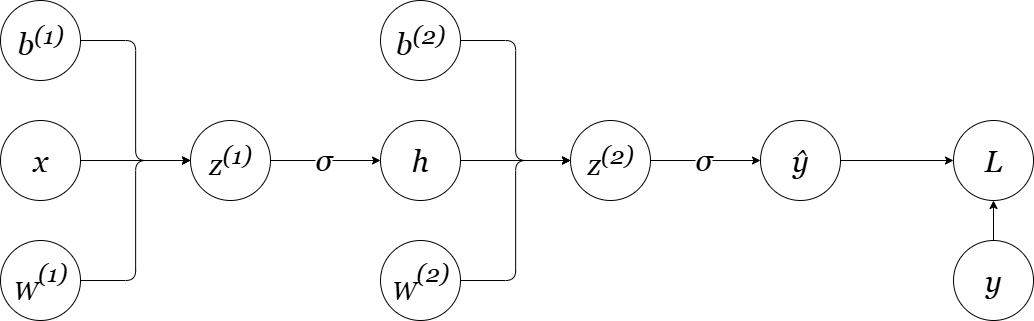
The real power of backpropagation emerges when we stack multiple layers. Let's consider a two-layer network and see how gradients flow backward through the computational graph.
Figure 3: A 2-layer multi-layer network
Note on Notation: As we generalize from a single neuron to a full layer of neurons, our parameters also generalize. We'll now use an uppercase $W$ to represent the weight matrix for a layer. Lowercase variables like $x$, $h$, and $b$ will represent vectors (or scalars in the case of a single bias).
The key insight: $\frac{\partial z^{(2)}}{\partial h} = W^{(2)}$ represents how the hidden layer influences the output layer.
🌟 The Recursive Pattern
Notice the elegant structure: to compute gradients for layer $\ell$, we need the gradients from layer $\ell+1$. This creates a natural recursive algorithm that processes layers in reverse order—the essence of backpropagation.
Multiple Neurons: Vectorization Emerges
When we have multiple neurons per layer, something beautiful happens: the individual gradient computations combine into elegant matrix operations. This is where the computational efficiency of backpropagation truly shines.
Matrix Formulation
Consider a hidden layer with $n$ neurons and an output layer with $m$ neurons. Our weight matrices become:
This vectorized form reveals the computational elegance: what could be hundreds of individual derivative calculations becomes just a few matrix multiplications!
Batch Processing: The Final Optimization
In practice, we rarely train on single examples. Instead, we process mini-batches of data simultaneously, which provides both computational efficiency and better gradient estimates.
Batch Dimensions
When processing a batch of $B$ examples, our tensors expand to include a batch dimension:
Input batch: $X \in \mathbb{R}^{B \times d}$ (B examples, d features each)
Hidden activations: $H \in \mathbb{R}^{B \times n}$ (B examples, n hidden units each)
Batch processing provides three key advantages: (1) Computational efficiency through vectorized operations, (2) Better gradient estimates by averaging over multiple examples, and (3) Memory efficiency by amortizing the cost of loading data and computing activations.
The General Backpropagation Algorithm
Now we can state the general backpropagation algorithm for an $L$-layer neural network processing mini-batches:
Algorithm: Mini-batch Backpropagation
Input: Training batch $(X, Y)$, network parameters $\{W^{(\ell)}, \mathbf{b}^{(\ell)}\}_{\ell=1}^L$
A complete, pedagogical implementation of the concepts discussed here—from single neurons to full networks with batch processing—is available on GitHub. The code includes detailed comments explaining each step of the forward and backward passes.